By
Motivation
When designing algorithms we want them to be as flexible as possible such that they can solve as many problems as possible. To solve a specific family of problems well, finding well-performing hyperparameter configurations requires us to either use extensive domain knowledge or resources. The second point is especially true if we want to use algorithms that we did not author ourselves. We most likely know nothing of the internals of the algorithm, so to figure out what makes this black-box tick, far too often, researchers of all flavors fall back to “Graduate Student Descent”.
Automated hyperparameter optimization and algorithm configuration offer far better alternatives, allowing for more structured and less error-prone optimization in potentially infinitely large search spaces. Throughout the search, various useful statistics are logged which can further allow us to gain insights into the algorithm, it’s hyperparameters and tasks the algorithm has to solve. At the end of the search, they present us with a hyperparameter configuration that was found to work well, e.g quickly finds a solution or has the best solution quality.
However the resulting static configurations these approaches are able to find exhibit two shortcomings:
- The configuration will only work well when the configured algorithm will be used to solve similar tasks.
- The iterative nature of most algorithms is ignored and a configuration is assumed to work best at each iteration of the algorithm.
To address Shortcoming 1, a combination of algorithm configuration and algorithm selection can be used. First search for well-performing but potentially complementary configurations (which solve different problems best) and then learn a selection mechanism to determine with which configuration to solve a problem. However, even this more general form of optimization (called per-instance algorithm configuration) is not able to address Shortcoming 2.
From Black-Box to White-Box
Classical approaches to configuration treat algorithms as black-boxes. When interacting with a black-box ƒ, we give it some input χ and observe the output γ it produces. We however can’t see inside the box. We can observe various different inputs and their corresponding outputs. We can use this data to learn what χ might produce the best γ.
Now if the box is an iterative system that processes χ over many stages, with the black-box view, we can only learn which input works well across all stages on average.
To be able to decide if a hyperparameter configuration is optimal at a given stage, we need some idea of how the algorithm behaves. We need to peer into the box. We can do this by tracking how the algorithm we want to optimize has interacted with a problem it has to solve. This information can then be used to learn how we need to adjust the hyperparameter configuration at each time-step.

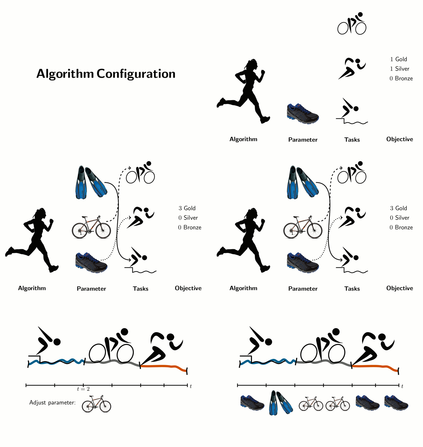
Comparison of different flavors of Algorithm Configuration. Dynamic Algorithm Configuration subsumes the prior frameworks. (Image credits: see bottom of the post)
Exemplary Applications of DAC
To illustrate the problem we will examine exemplary use-cases for dynamic algorithm configuration.
Learning rate schedules
A well known example of hyperparameters that need to be adjusted over time comes from deep learning. We know that static learning rates can lead to sub-optimal training times and results. Various schedules and adaptation schemes have been proposed, all with their individual merits and shortcomings. Using dynamic algorithm configuration, we could leverage some feedback about the learning-process to determine how we need to change a learning rate, not only over time but also according to the dataset we want to train a DNN on.
Restarting SLS solvers for SAT
Restarting, if done correctly, can allow to balance exploration and exploitation when solving problems in propositional satisfiability solving with stochastic local search solver. A restart means to start the search for a satisfying assignment anew from a new location in the search space. If the frequency of restarts is too high, finding a satisfying assignment might become impossible. On the other hand, if they occur too infrequent, a solver might spend too much resources evaluating unsolvable partial solutions. Depending on the problem a solver is facing, different schedules should be used.
Scheduling heuristics for AI planning
During planning, an AI planning system traverses potentially highly different search landscapes. As heuristics play a crucial role in guiding the system in how to traverse through these different spaces, different heuristics might be better suited as guides. Again, dynamic algorithm configuration allows to learn for which type of problems as well in which situations a heuristic should be chosen. (2021 update: Checkout our ICAPS’21 paper on this topic)
Step Size of Evolutionary Algorithms
In evolutionary algorithms, the step size guides how fast or slow a population traverses through a search space. Large steps allow to quickly skip over uninteresting areas, whereas small steps allow a more focused traversal of interesting areas. Handcrafted heuristics, are usually used trade-off small and large steps given some measure of progress. Directly learning in which situation which step-size is preferable allows dynamic algorithm configuration to act more flexible than a hand-crafted heuristic could. (2021 update: Checkout our PPSN’20 paper on this topic)
Dynamic Algorithm Configuration
Having discussed different potential applications and prior approaches, we can now discuss how dynamic algorithm configuration (DAC) can be applied and how it generalizes over the prior approaches. The crucial idea is that we have to stop treating algorithms as black-boxes. Using a gray-/white-box view on algorithms, we can formulate the optimization process as a Markov Decision Process (MDP), that models how an algorithm progresses given its parameterization.
An MDP is a 4-tuple M=(S, A, T, R) consisting of a state space S describing the algorithm state, an action space A changing the algorithm’s hyperparameter settings, a probability distribution T of algorithm state transitions, and a reward function R indicating the progress of the algorithm.
However, we still need to take into account that algorithms should solve many different problems. To encode this, we propose to use contextual MDPs instead. A contextual MDP MI={Mi}i~I induces multiple MDPs with shared state and action spaces, but with different transition functions and reward functions.
Imagine an algorithm has to solve two complementary problems. Configurations that enable quick progress on the first problem will most likely hinder progress on the second problem, which is reflected by the transition function and the reward function accordingly.
We expect that generally we won’t be able to model the transition function directly. However we don’t need to. Using reinforcement learning, we can still learn meaningful dynamic configuration policies directly from observed state, action and reward triples.

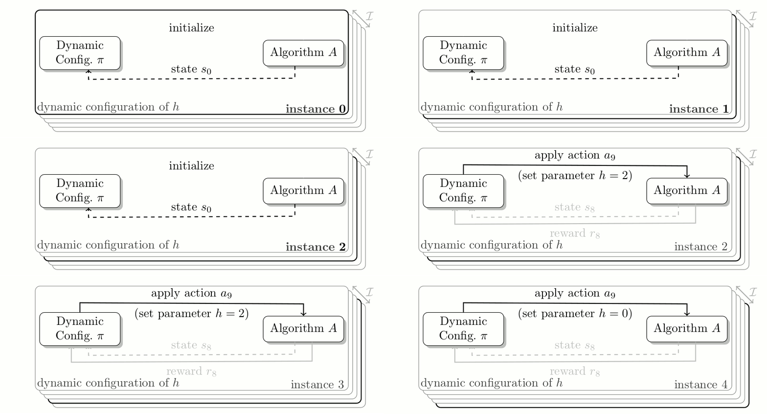
Algorithm Configuration as contextual Reinforcement Learning Problem. At each time step the configuration policy adjusts the value of hyperparameter h to optimize the reward at the current time step, whilst solving a given task.
Internally many algorithms track various statistics which are either directly used to decide on the behavior for the next (few) iteration(s) or to help developers debug/understand their algorithm. We argue that these statistics can be used to inform a dynamic configuration policy of how to adjust the configuration online. Furthermore, to allow the policy to adjust configurations depending on the problem, we propose to use the same descriptive features that have been used for algorithm selection.
Similarly, any statistic that informs us about the progress of the algorithm, is a suitable candidate as a reward signal. For example, the accuracy of a partially trained neural network could be used as a dense (i.e. available at every step) reward signal; whereas runtime could be a delayed reward signal (i.e., only available at the end).
In the above graphic, you see how a configuration policy interacts with an algorithm over a set of problem instances. At each time step the algorithm informs the policy of the internal state, and an incurred reward for using a given configuration. Based on this information, the dynamic configuration policy adjusts the hyperparameter.
Experimental Evaluation
In our recent paper, we evaluated our dynamic approach on benchmarks that exhibit a variety of factors that make dynamic configuration difficult.
If we choose the wrong hyperparameter settings at each time-step we might take many more steps to solve a problem, compared to choosing the best settings. We show that dynamic configuration policies can learn to handle such cases, solving a given problem in as few steps as possible.
Noisy reward signals pose a problem for general reinforcement learning agents. The noisier the signal, the harder the learning task. We show that, even though such an agent has to learn to average out the noise for each state individually, our proposed dynamic configurator is able to handle noisy signals fairly well, outperforming classical configuration in anytime and final performance.
As one of the goals of dynamic configuration policies is not only to adapt hyperparameters over time, but to also adapt them to the problem at hand, we evaluate our approach for varying degrees of homogeneity of the set/distribution of instances and how it can handle unseen problems. Using information about the problem at hand, our approach is able to infer if policies that work for a specific type of problem can be used for similar tasks, where the degree of homogeneity determines for how many problems the same policy can be reused. However, to generalize to unseen problems, we need to make use of function approximation.
Finally, most algorithms have many configurable hyperparameters. How these hyperparameters interact with each-other is often hard to gauge. To see how well out-of-the-box reinforcement learning agents can handle such spaces where the hyperparameters are strongly interacting, we evaluate our approach on a growing configuration space. We observe that, given strong interaction effects, that out-of-the-box agents struggle with handling such configuration spaces. However, our approach is still able to outperform the best static solutions found in the configuration spaces.
Take Home Message
Hyperparameter optimization is a powerful approach to achieve the best performance on many different problems. However classical approaches to solve this problem all ignore the iterative nature of many algorithms. Our new framework is capable of generalizing over prior optimization approaches, as well as handling optimization of hyperparameters that need to be adjusted over multiple time-steps. To allow us to use this framework, we need to move from the classical view of algorithms as a black-box to more of a gray or even white-box view to unleash the full potential of AI algorithms with DAC.
If you want to know more, check out the paper and the code.
Image Credits
- Female Runner (by algotruneman under CC0 1.0)
- Running Shoe (under CC BY-NC 4.0)
- Bike (under CC BY-NC 4.0)
- Flippers (under CC BY-NC 4.0)
- Cycling Pictogram (by Parutakupiu & Thadius856 under public domain)
- Athletics Pictogram (by Parutakupiu & Thadius856 under public domain)
- Swimming Pictogram (by Parutakupiu & Thadius856 under public domain)
- The above images were combined in gif form as abstract representations of different versions of Algorithm Configuration

